Field of Financial Optimization
It was already in 1952 that Harry Markowitz laid the foundation for the so called Mean-Variance-Analysis. When creating portfolios he evaluated stocks and securities, not only according to their returns, but took the variances and covariances into account as well. This approach results in the basic single-stage optimization problem which maximizes the portfolio return under a given restriction of the risk. In this formulation, only the first two moments of a distribution are considered. The mean describes the return and the variance is a measure for the risk.
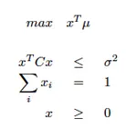
Solving this optimization problem for different risk levels (σ^2), one gets the set of all efficient portfolios, illustrated here in the μ-σ-plot.
In practice, there are often additional constraints required, e.g.
- allowance/permission of short selling
- additional restrictions of weights in sectors, countries, single positions
- limitation of the number of positions within the portfolio
- consideration of transaction costs
Starting from the above optimization program, one can formulate models for various problems like e.g. portfolio optimization relative to a benchmark or minimization of tracking error.
But this simple model by Markowitz also has some disadvantages. It is a single-stage optimization problem (consideration of only two points in time) which is often insufficient in practice: for example one is interested in optimal investment strategies over time, i.e. not only the actual asset allocation is relevant, but also the potential re-allocation of the portfolio in the course of time. Such a problem leads to multi-stage dynamic optimization.
Additionally, the results of the Markowitz optimization are very sensitive with respect to the input data, which is why more robust solutions and solution methods are wanted. For this question there exist several approaches.
The model of Markowitz takes only the first two moments of a distribution into account. Under the assumption that the returns of the considered securities in the optimization follow a normal distribution, the first two moments suffice to characterize the whole distribution. In practice, not only securities are considered for which such an assumption of the normal distribution is acceptable, but there can also be generated portfolios with clearly asymmetric distributions, e.g. by adding options. That means expectation and variance are not sufficient to characterize the whole distribution.and an optimization based on these two first moments is not adequate.
Variance is a measure for the variation around the expected value – in both directions. Since only losses represent a real risk, the variance is not the ideal risk measure. When measuring risk in finance, the shortfall (the fact of not reaching a given benchmark) is more important. The shortfall condition can be seen as another risk measure. This leads to stochastic optimization with a constraint that the probability of losses is less than a % or that the expected loss does not exceed a certain amount.
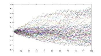
Regarding complex portfolio structures or distributions or regarding investment strategies over time, return and risk often cannot be stated as a closed formula. In such a case simulations of scenarios can be used as a basis for the optimization.
Using models for the different financial markets, the asset classes are simulated consistently over time. Based on these scenario paths, different portfolios or investment strategies are calculated, from which the “optimal” strategy can be estimated.
We can illustrate scenario simulation as follows.
Current topics at the Chair of Mathematical Finance in the field of financial optimization are
- improvement of the robustness of solutions of optimization problems using different approaches
- including forecasts of experts into the optimization
- using genetic methods for solving portfolio optimization problems
- optimization of investment strategies