The Surrogate Matrix Methodology

We revisit the classical lowest-order Bubnov-Galerkin finite element method and analyze a modification of it which is strongly amenable to stencil-based matrix-free computation. Roughly speaking, it requires performing quadrature for only a small fraction of the trial and test basis function interactions and then approximating the rest through, for example, interpolation. The main idea was first introduced in the context of first-order finite elements in [Bauer et al., 2017]. Thereafter, applications to peta-scale geodynamical simulations were presented in [Bauer et al., 2019] and a theoretical analysis was given in [Drzisga et al., 2018]. In the massively parallel applications, it is natural to work with so-called macro-meshes as well as a piecewise polynomial space for resolving the surrogate matrices. Recently, we presented a simple methodology to avoid over-assembling matrices in Isogeometric Analysis in [Drzisga et al., 2019]. In contrast, the surrogate matrices in this work are computed using a B-spline interpolation space.

Problem Setting and Motivation

Let $V$ be a suitable space and $V_h\subsetneq V$be a finite-dimensional subspace.
Consider a bilinear form $a$, its surrogate bilinear form $\tilde{a}$, and a linear functional $F$.
Many physical problems may be written in the form
$$\begin{equation}
    \text{Find } u_h \in V_h \text{ satisfying }

    \quad
    a(u_h,v_h)
     =
    F(v_h)
    \quad
      \text{for all } v_h\in V_h
\\
    \text{Find } \tilde{u}_h \in V_h \text{ satisfying }

    \quad
    \tilde{a}(\tilde{u}_h,v_h)
     =
    F(v_h)
    \quad
      \text{for all } v_h\in V_h
\end{equation}$$
These discrete variational problems induce matrix equations of the form
$Au = f$ and $\tilde{A}\tilde{u} = f$.
The surrogate matrix $\tilde{A}$should satisfy following properties:
   * $\tilde{A}$ should be as close as possible to the standard matrix $A$
   * $\tilde{A}$ should be computationally cheaper to obtain than $A$
   * $\tilde{A}$ should preserve properties of the standard matrix $A$, e.g., symmetry

Stencil functions

Assume that the bilinear form is of the form
$$\begin{equation*}
a(u,v) = \int_\Omega G(x,u(x),v(x)) \mathrm{d} x
\qquad \text{for all } u, v\in V,
\end{equation*}$$
e.g., Poisson problem for $G(x,u,v) = {\nabla u^\top K(x) \nabla v}$ and \(K = \frac{D\varphi^{-1} D\varphi^{-\top}}{|\det{\left(D\varphi^{-1}\right)}|}\(.

Let $\phi\in V$ be a test function and $\phi_\delta(x) = \phi(x-\delta)$. We define the stencil function $\Phi^\delta(x)$ with a shift $\delta$ as
$$\begin{equation*}
\Phi^\delta(x) := \int_{\Omega_{\delta}} \!\!G(x+y,\phi(y),\phi_{\delta}(y)) \,\mathrm{d} y
\end{equation*}$$

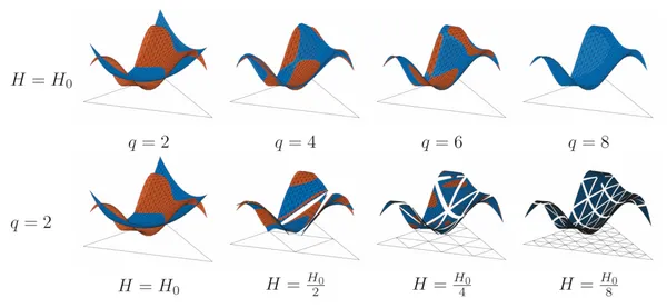
Observe that the stencil functions $\Phi^\delta$ are smooth functions, as can be seen in the picture below.
Therefore, replace stencil functions by surrogates which allow fast evaluation: $\tilde{\Phi}^\delta = \Pi^\delta\, \Phi^\delta$

If $x_j - x_i = \delta$, observe that
$A_{ij} = a(\phi_j, \phi_i) = \Phi^\delta(x_i)$
For semi-structured meshes, the set $\mathcal{D}(x_i) = \{x_j-x_i \,:\, \, a(\phi_{j},\phi_{i}) \neq 0\}$ is small, thus only a small number of stencil functions is required to describe the whole matrix.

With $\tilde{\Phi}^\delta = \Pi^\delta\, \Phi^\delta$, we thus define the surrogate matrix as
$$\begin{equation*}
\tilde{A}_{ij}
=
\begin{cases}
\tilde{\Phi}_\delta(x_i) & \text{if } x_i,x_j\in\tilde{\Omega},
\\ A_{ij} &\text{otherwise.}
\end{cases}
\end{equation*}$$
This definition may be easily extended to preserve symmetries and kernels of $A$.

Results

$p$-Laplacian diffusion example

We considered the time-dependent non-linear $p$-Laplacian diffusion problem, given in strong form as
$$\begin{equation}
\begin{alignedat}{2}
\frac{\partial u}{\partial t} - \mathrm{div}\left(|\nabla u|^{p-2} \cdot u\right) &= f &&\quad \text{in } \Omega \times (0,T_{\mathrm{end}}]\,,
\\ u &= 0 &&\quad \text{on } \partial \Omega \times (0,T_{\mathrm{end}}]\,, \\
\\ u &= u_0 &&\quad \text{in } \Omega \times \{0\}\,.
\end{alignedat}
\end{equation}$$

Stokes' lid driven cavity flow in deformed domain

We consider a lid-driven cavity benchmark on a deformed domain where the fluid satisfies following equations:

$$\begin{equation*}
\begin{alignedat}{2}
-\Delta u + \nabla p &= f &&\quad \text{in } \Omega,
\\ \mathrm{div}(u) &= 0 &&\quad \text{in } \Omega,
\\ u &= g &&\quad \text{on } \Gamma_{\text{D}}
\end{alignedat}
\end{equation*}$$

In this scenario the fluid is driven on the top edge by constant velocity $g = (1,0)^\top$ and we assume no-slip boundary conditions $g = 0$ on the remaining parts of the boundary.
The degrees of freedom corresponding to the nodal basis functions in the top left and top right corner are set to zero.
Furthermore, the volume forces are neglected, i.e., $f = 0$.
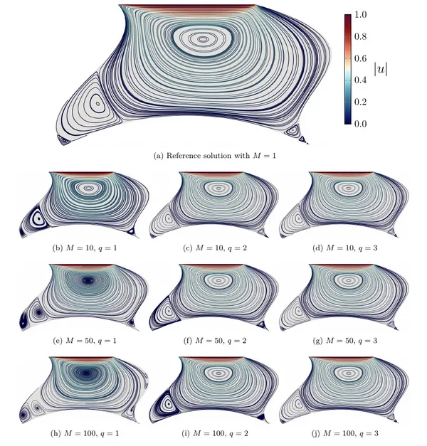
Below, we show the velocity streamlines which were computed using a standard IGA approach on a mesh with $320 \times 320$ control points.
Furthermore, the effect of different surrogate approaches on the velocity streamlines may be observed.
In the case where the interpolation order is given by $q = 3$, the streamlines show the same behavior as in the standard approach even for a skip paramater $M = 100$.
For other values of $q$ and $M$, the streamline behavior is different, but the streamlines are getting closer to the reference solution the larger $q$ and the smaller $M$ becomes.
We note that actually using an interpolation order of $q=1,2,3$ in computation is still probably not recommended for standard practice.
For instance, assembly using $q=5$ took roughly the same time as either of these lower-order choices and, in this case, the surrogate solution should be expected to be even more accurate.

Publications

(Keine Dokumente in dieser Ansicht)