- Avoiding Pyrolysis and Calcination: Advances in the Benign Routes Leading to MOF2̆010Derived Electrocatalysts. ChemElectroChem 9 (7), 2022 mehr…
Blood flow simulation
Modeling of blood flow and transport at the level of microcirculation is an interesting subfield in biomedical engineering. A reliable computational model for the microcirculation of the human body would enable physicians and pharmacists to obtain better insight into the oxygen supply of cells, the waste removal from the interstitial space and further important biological processes without the need to perform expensive and risky experiments. Such simulations can be really expensive to perform. In fact, even for vascular systems contained in small volumes covering just a few cubic millimetres, it is a challenging task to simulate flow in the microvascular networks and the interstitial space, since the flow in a complex network structure consisting of thousands of vessels is coupled with the flow in the surrounding tissue. To reduce the computational complexity of this issue, the network structures are modeled by a one-dimensional graph, whose location in space is determined by the centerlines of the three-dimensional vessels. The topics we investigate at our Chair regard the analysis and implementation of different coupling strategies between the one-dimensional network and the three-dimensional medium. Furthermore, such strategies are used to simulate flow and transport in realistic vascular system.
Problem Setting
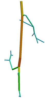
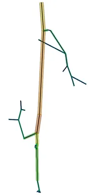
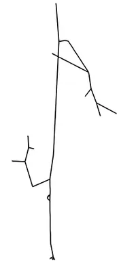
The first step of blood flow simulation consists in the generation of the one-dimensional network representing the vascular structure, having the three-dimensional one at hand. The next figure shows the procedure to obtain of a vascular graph model for an arteriole. On the left, the arteriole is fully resolved and approximated by cylinders. In the middle, the centerlines are depicted and on the right, the vascular graph model for the arteriole is extracted.
Under specific assumptions, the model used to describe the blood flow in the microvascular network is given by Poiseuille’s law for conservation of momentum and mass combined with a standard diffusion model and Darcy's law for the flow in the surrounding tissue. The interaction between the vascular system and the tissue is described by the standard Starling's filtration law. All in all, we obtain the following type of equations:
$$
-\nabla \cdot \left( \rho_{\mathrm{int}} \frac{K_{\mathrm{t}}}{\mu_{\mathrm{int}}} \nabla u^{\mathrm{t}}\right)=
L_{\mathrm{cap}} \rho_{\mathrm{int}} \left(u^{\mathrm{v}}-\overline{u^{\mathrm{t}}} - \left( \pi_{\mathrm{p}} - \pi_{\mathrm{int}} \right) \right)\delta_{\Gamma}, \quad \text{in } \Omega,
$$
$$
-\frac{d}{ds}\left( \rho_{\mathrm{bl}} \pi R^2 \frac{K_{\mathrm{v}}}{\mu_{\mathrm{bl}}} \frac{du^{\mathrm{v}}}{ds} \right)=
2 \pi R L_{\mathrm{cap}} \rho_{\mathrm{int}} \left(\overline{u^{\mathrm{t}}}-u^{\mathrm{v}} + \left( \pi_{\mathrm{p}} - \pi_{\mathrm{int}} \right)\right), \quad \text{in } \Lambda.
$$
A selection of results
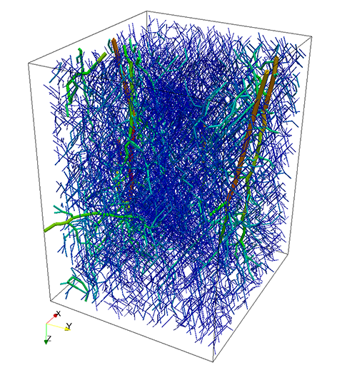
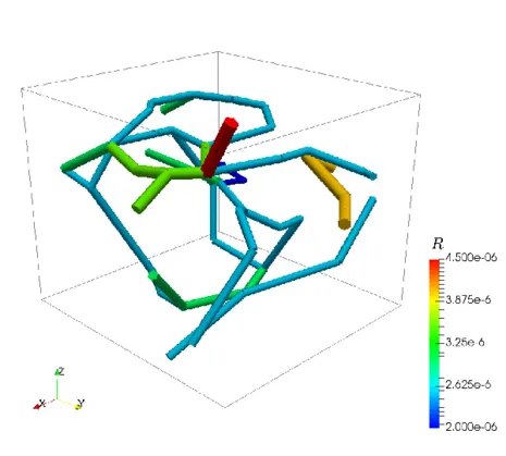
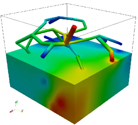
As an idealized application, let us consider a prototype model for stationary flow in biological tissue supplied by a network of capillaries. The network is available here and is depicted on the left figure. In particular, it represents a portion of a rat cerebral cortex and consists of a relatively small set of microvessels and is depicted on the left. The 3D-1D coupled problem presented above is solved by means of a linear finite elements approximation. In the middle figure, the numerical approximations of both pressures (in the network and in the tissue) is presented, where we can notice that the solution in the tissue appears to behave in accordance to the solution in the network. In the right figure, plasma fluid paths from high-pressure capillaries to low-pressure capillaries through the interstitial space for the 3D-1D coupled problem are depicted.
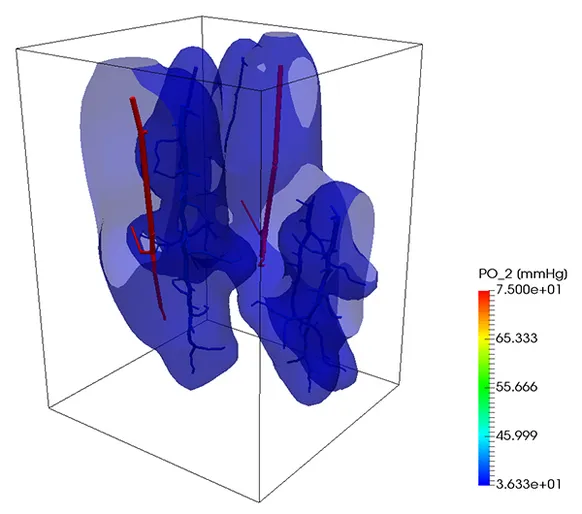
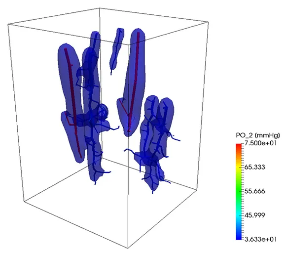
Oxygen transport
A similar strategy can be also used to simulate the transport of a substance trough the vascular system into the tissue. In the next example, oxygen is transported trough the vascular system and exchanged with the tissue, which consumes it at a given rate. So, if the portion of the tissue is not enough covered by the vascular system, the oxygen level lowers, causing the death of the tissue. At the beginning of the simulation, the tissue was set to have a given oxygen concentration corresponding to a partial pressure of 50 mmHg. After 9 seconds, the contour level of oxygen corresponding to a partial pressure of 2 mmHg is depicted. On the right figure, the same contour level is depicted after one minute.