(Keine Dokumente in dieser Ansicht)
High Performance Computing
Current state of the art supercomputers perform several petaflops and thus enable large-scale simulations of physical phenomena. The enormous computational power is particularly valuable when large computational domains must be resolved with a fine mesh. For minimizing the resource consumption in, e.g., compute time, processor numbers, memory, or energy, we must proceed beyond the demonstration of asymptotic optimality for the algorithms and beyond establishing the scalability of the software. Modern fast solvers must additionally be implemented with data structures that permit an efficient execution on multicore architectures exploiting their instruction level parallelism, and they must be also adapted to the complex hierarchical memory structure.This necessitates a meticulous efficiency-aware software design and an advanced performance aware implementation technology.
Interdisciplinary work
The presented work requires a careful co-design and expertise of many disciplines and can not be stemmed by mathematicians alone. Therefore, we interdisciplinarily work with the following partners from computer science and geophysics and their corresponding research associates and students
- Prof. Dr. Ulrich Rüde: Head of the Chair of Computer Science 10 (System Simulation) at the Friedrich–Alexander University Erlangen–Nürnberg
- Prof. Dr. Gerhard Wellein: Professorship for High Performance Computing at the Friedrich–Alexander University Erlangen–Nürnberg
- Prof. Dr. Hans-Peter Bunge: Professorship for Geophysics at the Ludwig Maximilian University of Munich
Problem setting and motivation
Stokes Solvers
We studied the performance of different, existing solution algorithms and their influence on different formulations of the Stokes system, which include the Laplace- or the divergence of the symmetric part of the gradient operator. Iterative solution techniques for saddle point problems have a long history. In general, we distinguish between preconditioned iterative methods (Krylov subspace methods) and all-at-once multigrid methods where the multigrid algorithm is used as a solver for the saddle point problem. Both solver types were studied, and numerical examples illustrate that they perform with excellent scalability on massively parallel machines. In case of the all-at-once multigrid method, we reach up to 1013 degrees of freedom .
Resilience
The driving force behind the research interest in achieving larger computing systems with more than \(10^18\) floating point operations (FLOPS) per second (exa-scale) originates in the potentials to expand science and engineering by simulation. For the upcoming exa-scale computing era, expected in the next decade, the enormous increase in compute power also constitutes new grand challenges for these architectures. One of the key challenges will be building reliable systems with massively increasing components while keeping the energy consumption of the system low.
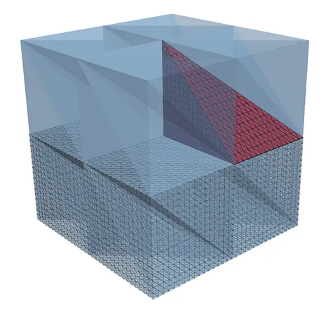
Fault tolerant massively parallel multigrid methods for elliptic partial differential equations are a step towards resilient solvers. For our study, we concentrate on a specific fault model and consider that faults of either a processor or a compute node. The data of the part of the computational domain \(\Omega\) which is lost due to the failure is called faulty domain \(\Omega_F\) (marked red). The subdomain \(\Omega_I = \Omega \backslash \Omega_F\) is called healthy or intact domain (marked blue). Further, we define the interface \(\Omega_\Gamma = \overline{\Omega}_F \cap \overline{\Omega}_I\), i.e., the nodes which have dependencies in the faulty and healthy domain are located on \(\Omega_\Gamma\).
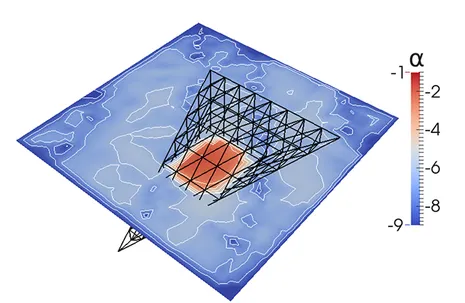

The middle illustration visualizes the residual on a cross section through the domain directly after the failure and re-initialization. The residual distribution when one additional global multigrid cycle has been performed is given on the right. Note that large local error components within ΩF are dispersed globally by the multigrid cycle. Although the smoother transports information only across a few neighboring mesh cells on each level, their combined contributions on all grid levels lead to a global pollution of the error. While the residual decreases globally, the residual in the healthy domain ΩΓ increases by this pollution effect. A possible remedy is based on temporarily decoupling the domains in order to avoid that the locally large residuals can pollute into the healthy domain.
Multilevel Monte Carlo
MLMC methods are characterized by three algorithmic levels that are potential candidates for parallel execution. As in standard Monte Carlo methods, a sequence of classical deterministic problems (samples) are solved that can be computed in parallel. Additionally one can distinguish between parallelism within an MLMC level and parallelism across MLMC levels. The third algorithmic parallelization level is the solver for the deterministic PDE problem. Indeed, the total number of samples on finer MLMC levels is typically moderate, so that the first two levels of parallelism will not suffice to exploit all available processors.We analyzed how these different levels of parallelism can be combined and how efficient parallel MLMC strategies can be designed.
Results
Stokes Solvers
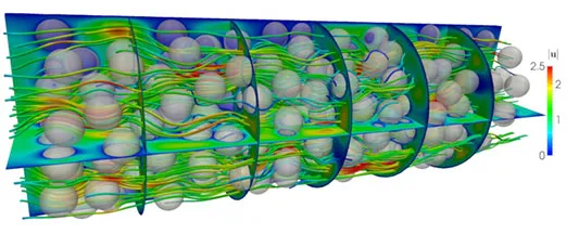
We considered as a computational domain, similar to a so-called packed sphere bed. We use a cylinder, aligned along the \(x_1\)-axis of length 6 and radius 1 with a given number, \(n = 305\) of spheres which are obstacles, i.e., the domain is \(\Omega = \{ \mathbf{x} \in \mathbb{R}^3\, :\, x_2^2 + x_3^2 < 1,\, x_3 \in (0, 6) \} \setminus \overline{\mathcal{B}}\), where \(\mathcal{B} = \bigcup_{i=1}^{n_s} B_r(\mathbf{c}_i)\) is the union of spheres with radius \(r = 0.15\) that are located at the center points \(\mathbf{c}_i \in \Omega\). The points \(\mathbf{c}_i\) are randomly chosen, have a minimal distance of \(2r\) from each other, and have at least a distance of \(r\) from the cylinder boundary. Note, spheres might have a very small distance to each other or the cylinder boundary, which makes the problem even more challenging.
The numerical results are performed with the Uzawa multigrid method, since it is the most efficient with respect to time-to-solution and memory consumption. For the computations, we consider the relative accuracy \(\epsilon = 10^{-5}\) and a zero initial vector. The initial mesh \(\mathcal{T}_{-2}\), representing the domain \(\Omega\), consists of approximately \(1.3 \cdot 10^5\) tetrahedrons. The initial mesh is then refined 5 times, i.e., the coarse grid consists of \(8.3 \cdot 10^6\) tetrahedrons and the resulting algebraic system on the finest mesh consists of about \(2.7 \cdot 10^9\) degrees of freedom.
Resilience
In the case of a fault, the redundant interface values can be easily recovered while the lost inner unknowns are re-computed approximately with recovery algorithms using multigrid cycles for solving a local Dirichlet problem. Different strategies are compared and evaluated with respect to performance, computational cost, and speed up. Especially effective are asynchronous strategies combining global solves with accelerated local recovery.
The computations in both the faulty and healthy subdomains must be coordinated in a sensitive way, in particular, both under- and over-solving must be avoided. Both of these waste computational resources and will therefore increase the overall time-to-solution. To control the local recovery and guarantee an optimal re-coupling, we introduce a stopping criterion based on a mathematical error estimator. It involves hierarchically weighted sums of residuals within the context of uniformly refined meshes and is well-suited in the context of parallel high-performance computing. The re-coupling process is steered by local contributions of the error estimator before the fault.
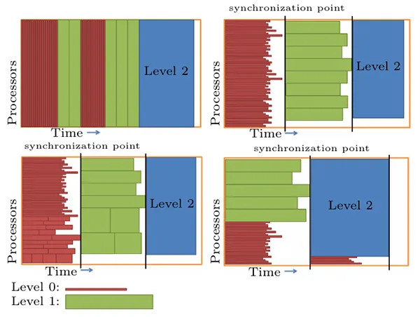
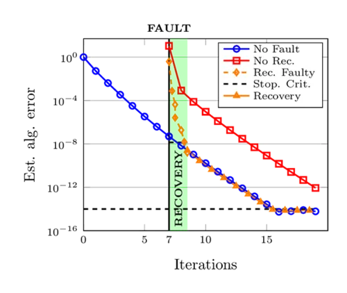
The input mesh in our first experiment is the unit cube discretized by 24576 tetrahedrons, which results after uniform refinement in a linear system with 1.3·108 DOFs. To load-balance the problem, we run these simulations with 48 MPI-processes and assign to each process 512(= 83) input mesh tetrahedrons. We use in the re-coupling criterion the bound σLRB and κ=1.0 for the two superman acceleration factors ηs = 2 and η s = 4. In he fowollowing Figure 8, we present the estimated algebraic error within a faulty solution process. The plots left and right refer to ηs=2 and ηs=4, respectively. In order to satisfy the re-coupling criterion, 6 local multigrid iterations are necessary in the faulty subdomain which can be performed simultaneously while 3.7 and 2.0 iterations are executed in the healthy domain, respectively, depending on the superman acceleration ηs. In the faulty domain, the error estimator is applied in addition to the V-cycles. Asynchronously, the computations in the healthy domain are executed. The recovery process is highlighted in light green in the figures. Note, that fractional numbers imply that the healthy domain receives the stopping signal for re-coupling when the multigrid iteration in the healthy domain has not completed the most recent cycle. So for example, when the healthy domain has executed the downward branch of a symmetric V-cycle, we will have executed one half of a V-cycle and denote this in the following tables and graphics by 0.5 iterations. Summarizing our experiments, we find that the recovery with ηs=2 results in a delay of only up to three iterations and with ηs=4 in up a delay of two iterations. Thus, the adaptive re-coupling strategy reduces significantly the costs in comparison to applying no recovery strategy.
Multilevel Monte Carlo
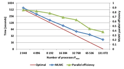
We performed strong scaling experiments of MLMC using homogeneous bulk synchronous scheduling with up to 131072 of processes. Increasing the number of processes while keeping the number of samples per level fixed results in an increased load imbalance and the total parallel efficiency decreases. Nevertheless, even with 32768 processes, we obtain a parallel efficiency of over 60%. For 131072 processes, the efficiency drops below 40%, since we have reached the limits of the scalability window. This is inevitable in any strong scaling scenario. Overall, the compute time for the MLMC estimator can be reduced from 616 to 22 seconds, resulting in an excellent parallel efficiency of the MLMC implementation.
Publications
(Keine Dokumente in dieser Ansicht)