(Keine Dokumente in dieser Ansicht)
Uncertainty Quantification and Bayesian inversion for complex models
Problem Setting and Motivation
Many physical models are parameterized, in the sense that they need a set of model parameters for the description of a complex phenomenon. Parameters comprise, e.g., scalar values like the viscosity in a CFD simulation or function values like boundary conditions in PDE models. All of them are often not known a priori without further investigation. The field of Uncertainty Quantification (UQ) provides methods to gain information about parameter values and their uncertainties.
Bayesian inverse problems are, within the field of UQ, a popular approach to formulate well-posed inverse problems. The goal in a Bayesian inverse problem is the approximation of a posterior distribution \(\mu_d\), or, short, posterior, on the space of parameters. The posterior is a distribution that is conditioned on the observation of a particular measured data set \(d\), i.e., $$\mu_d = \mathbf{P}(\lbrace x \in \cdot | d = \mathcal{G}(x) + \eta\rbrace),$$ where \(\mathcal{G}\) is the parameter-to-observation operator and \(\eta\sim\mathcal{N}(0,\Gamma)\) models additive Gaussian noise with covariance matrix \(\Gamma\). By Bayes' Theorem, the posterior is also dependent on a prior distribution \(\mu_0\). The prior serves as a regularizer to the problem and is supposed to be a first guess on the distribution of the model parameters.
Bayesian inversion is sometimes also called Bayesian updating since the prior is "updated" by the incorporation of data to become a posterior. Constructing samples of the posterior is not trivial and can get computationally expensive. Especially if the model runs are costly and the parameter space is high-dimensional, the construction of (uncorrelated) posterior samples can be intractable. Common techniques for the generation of posterior samples are, e.g., Importance Sampling, Sequential Monte Carlo (SMC), and Markov chain Monte Carlo (MCMC).
We are utilizing MCMC algorithms that are based on the popular Metropolis-Hastings algorithm, which constructs a Markov chain whose stationary distribution is the posterior. It is known that Metropolis-Hastings, although it does not suffer from the curse of dimensionality as much as other samplers, has deteriorating properties in high-dimensional spaces like, e.g., an bad mixing behavior of the constructed Markov chain. Hence, reducing the dimension of a Bayesian inverse problem can speed up computations by orders of magnitude. For this purpose, we are applying a recent approach called the active subspace method.
Results
Active subspaces for Bayesian inversion
Active subspaces is an emerging set of tools for dimension reduction; see e.g. Constantine et al., 2014.
This technique tries to find a low-dimensional approximation \(g\,:\mathbf{R}^k\to\mathbf{R}\) to a high-dimensional function \(f \mathbf{R}^n\to\mathbf{R}\), where \(k \ll n\).
Consider, for example, a function \(f\) of the form$$f(x) = g(A^\top x),$$ where \(A\in\mathbf{R}^{n\times k}\), \(k<n\).
Such functions are called ridge functions , see for example the following figure:
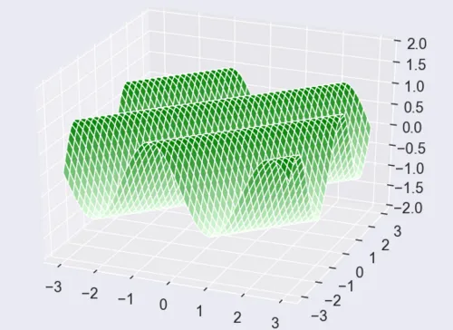
Ridge functions change their value only along a subspace, namely along the null space of \(A^\top\), since, for \(v \in N(A^\top)\), it holds that $$f(x+v) = g(A^\top(x+v)) = g(A^\top x) = f(x).$$
This means that, for more general \(f\), if we are able to find directions, along which \(f\) varies dominantly, we can hope to find a good approximation \(g(A^\top x) \approx f(x)\).
Dominant directions are studied with the eigendecomposition of $$C = \int {\mathbf{R}^n}{\nabla f(x)\nabla f(x)^\top \, \rho(x) \, dx} = W\Lambda W^\top.$$
The eigenvalues in \(\Lambda\) show (averaged) sensitivities in the direction of corresponding eigenvectors, since it holds that $$\lambda i = w i^\top Cw i = \int {\mathbf{R}^n}{(w i^\top\nabla f(x))^2\,\rho(x)\,dx}.$$
Hence, if we split \(W\) accordingly, we can introduce new, transformed variables that are aligned to the dominant directions.
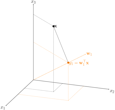
Indeed, we split $$W=[W 1\quad W 2]$$ and write $$x = WW^\top = W 1W 1^\top x + W 2W 2^\top x = W 1y+W 2z,$$ where \(y=W 1^\top x\) and \(z=W 2^\top x\) are called the active and, respectively, inactive variables.
The column space of \(W 1\) is called the active subspace (of \(f\)).
The figure below shows an example of an original 3-dimensional space with a 1-dimensional active subspace.
The function \(f\) that we aim to approximate low-dimensionally in the context of Bayesian inversion is the so-called data misfit function .
If we assume additive Gaussian noise in our Bayesian inverse problem (like above), then the (Lebesgue) density of the posterior is $$\rho d(x) = \rho d(x|d) \propto \exp(-f d(x))\,\rho 0(x),$$
where \(\rho 0\) is the (Lebesgue) density of the prior distribution \(\mu 0\) and \(f d(x):=\frac{1}{2}||d-\mathcal{G}(x)|| \Gamma^2\) is the data misfit function.
After finding the dominant directions, we are able to run our MCMC algorithms in lower dimensions which speeds up the construction of posterior examples.
We applied this procedure to two parameter studies of complex physical models, namely a nonlinear elasticity model for simulating the behavior of methane hydrates (see Teixeira Parente et al., 2018), and a hydrotope-based karst hydrological model simulating discharge values in the Kerschbaum spring area in Waidhofen a.d. Ybbs (see Teixeira Parente et al., 2019).
Other approaches that can be regarded as belonging to the field of Uncertainty Quantification and Bayesian inversion can be can be found in the publication list below.